10.1. Quality Assurance Checks for Successful CMAQ Run on CycleCloud#
10.1.1. run m3diff to compare the output data for two runs that have different values for NPCOL#
cd /shared/data/output
ls */*ACONC*
setenv AFILE output_v54_cb6r5_ae7_aq_WR413_MYR_gcc_2018_12US1_3x96/CCTM_ACONC_v54_cb6r5_ae7_aq_WR413_MYR_gcc_2018_12US1_3x96_20171222.nc
setenv BFILE output_v54_cb6r5_ae7_aq_WR413_MYR_gcc_2018_12US1_4x96/CCTM_ACONC_v54_cb6r5_ae7_aq_WR413_MYR_gcc_2018_12US1_4x96_20171222.nc
m3diff
hit return several times to accept the default options
grep A:B REPORT
Should see all zeros. There are some non-zero values. It appears to have all zeros if the domain decomposition is the same NPCOL, here, NPCOL differs (10 vs 16) Did a test to determine if removing the compiler option -march=native would result in zero differences if NPCOL differs. This seems to work on CycleCloud, but did not work on Parallel Cluster.
Verify that you have loaded the gcc and openmpi modules.
module avail
module load gcc-9.2.0
module load mpi/openmpi-4.1.5
Verfiy the compiler version:
gcc --version
Output
gcc (GCC) 9.2.0
Evaluation of the Makefiles on Cyclecloud:
cd /shared/build/openmpi_gcc/CMAQ_v54/CCTM/scripts/BLD_CCTM_v54_gcc
grep FSTD Makefile
Output (note there is no longer the option -march=native that was causing differences in answers:
FSTD = -O3 -funroll-loops -finit-character=32 -Wtabs -Wsurprising -ftree-vectorize -ftree-loop-if-convert -finline-limit=512
Check NPCOL NPROW for each run script
grep 'NPCOL =' run_cctm_2018_12US1_v54_cb6r5_ae6.20171222.3x96.ncclassic.csh
@ NPCOL = 16; @ NPROW = 18
grep 'NPCOL =' run_cctm_2018_12US1_v54_cb6r5_ae6.20171222.4x96.ncclassic.csh
Output
@ NPCOL = 16; @ NPROW = 24
grep A:B REPORT
output
 A:B  0.00000E+00@(  1,  0, 0)  0.00000E+00@(  1,  0, 0)  0.00000E+00  0.00000E+00
 A:B  0.00000E+00@(  1,  0, 0)  0.00000E+00@(  1,  0, 0)  0.00000E+00  0.00000E+00
 A:B  0.00000E+00@(  1,  0, 0)  0.00000E+00@(  1,  0, 0)  0.00000E+00  0.00000E+00
 A:B  0.00000E+00@(  1,  0, 0)  0.00000E+00@(  1,  0, 0)  0.00000E+00  0.00000E+00
 A:B  0.00000E+00@(  1,  0, 0)  0.00000E+00@(  1,  0, 0)  0.00000E+00  0.00000E+00
 A:B  0.00000E+00@(  1,  0, 0)  0.00000E+00@(  1,  0, 0)  0.00000E+00  0.00000E+00
 A:B  0.00000E+00@(  1,  0, 0)  0.00000E+00@(  1,  0, 0)  0.00000E+00  0.00000E+00
 A:B  0.00000E+00@(  1,  0, 0)  0.00000E+00@(  1,  0, 0)  0.00000E+00  0.00000E+00
 A:B  0.00000E+00@(  1,  0, 0)  0.00000E+00@(  1,  0, 0)  0.00000E+00  0.00000E+00
 A:B  0.00000E+00@(  1,  0, 0)  0.00000E+00@(  1,  0, 0)  0.00000E+00  0.00000E+00
 A:B  0.00000E+00@(  1,  0, 0)  0.00000E+00@(  1,  0, 0)  0.00000E+00  0.00000E+00
 A:B  0.00000E+00@(  1,  0, 0)  0.00000E+00@(  1,  0, 0)  0.00000E+00  0.00000E+00
 A:B  0.00000E+00@(  1,  0, 0)  0.00000E+00@(  1,  0, 0)  0.00000E+00  0.00000E+00
 A:B  0.00000E+00@(  1,  0, 0)  0.00000E+00@(  1,  0, 0)  0.00000E+00  0.00000E+00
 A:B  0.00000E+00@(  1,  0, 0)  0.00000E+00@(  1,  0, 0)  0.00000E+00  0.00000E+00
 A:B  0.00000E+00@(  1,  0, 0)  0.00000E+00@(  1,  0, 0)  0.00000E+00  0.00000E+00
 A:B  0.00000E+00@(  1,  0, 0)  0.00000E+00@(  1,  0, 0)  0.00000E+00  0.00000E+00
 A:B  0.00000E+00@(  1,  0, 0)  0.00000E+00@(  1,  0, 0)  0.00000E+00  0.00000E+00
 A:B  0.00000E+00@(  1,  0, 0)  0.00000E+00@(  1,  0, 0)  0.00000E+00  0.00000E+00
 A:B  0.00000E+00@(  1,  0, 0)  0.00000E+00@(  1,  0, 0)  0.00000E+00  0.00000E+00
 A:B  0.00000E+00@(  1,  0, 0)  0.00000E+00@(  1,  0, 0)  0.00000E+00  0.00000E+00
 A:B  0.00000E+00@(  1,  0, 0)  0.00000E+00@(  1,  0, 0)  0.00000E+00  0.00000E+00
 A:B  0.00000E+00@(  1,  0, 0)  0.00000E+00@(  1,  0, 0)  0.00000E+00  0.00000E+00
10.1.2. If CMAQ were compiled with -march=native, then you would see differences in the output if NPCOL was different, see previous version of this tutorial for more information#
10.2. R analysis scripts#
10.2.1. Run the following R script to create box plots and spatial plots showing difference between two CMAQ runs.#
Note: requires that the R scripts and packages. See earlier instructions.
edit the R script to specify the sim1.dir, sim1.file and sim2.dir, sim2.file to correspond to the Benchmark cases that have been run.
Then run the R scripts!
cd /shared/cyclecloud-cmaq/qa_scripts
Rscript compare_EQUATES_benchmark_output_CMAS_cyclecloud.r
Note, if you have a + symbol in the log filename, the script will fail. Rename 5.4+ to 5.4plus to use the scripts.
View the Operating System
cat /etc/os-release
Output:
NAME="CentOS Linux"
VERSION="7 (Core)"
ID="centos"
ID_LIKE="rhel fedora"
VERSION_ID="7"
PRETTY_NAME="CentOS Linux 7 (Core)"
ANSI_COLOR="0;31"
CPE_NAME="cpe:/o:centos:centos:7"
HOME_URL="https://www.centos.org/"
BUG_REPORT_URL="https://bugs.centos.org/"

CENTOS_MANTISBT_PROJECT="CentOS-7"
CENTOS_MANTISBT_PROJECT_VERSION="7"
REDHAT_SUPPORT_PRODUCT="centos"
REDHAT_SUPPORT_PRODUCT_VERSION="7"
Example output plots are available for the CONUS Benchmark in the following directory
When NPCOL is fixed, we are seeing no difference in the answers.
Example comparison of 10x18 compared to 9x10 with the -march=native compiler flag removed
Box Plot for ANO3J when -march=native compiler flag is removed
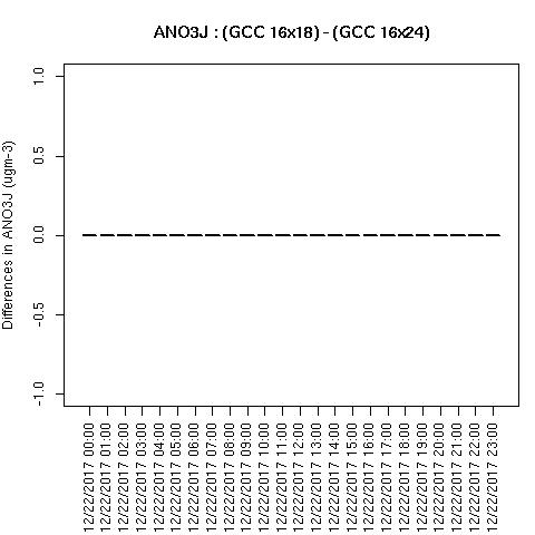
Box plot shows no difference between ACONC output for a CMAQv5.4 run using different PE configurations as long as NPCOL is fixed (this is true for all species that were plotted (AOTHRJ, CO, NH3, NO2, O3, OH, SO2), or when not using march=native in the compiler flag
Spatial plots were not created by the script, as there were not differences between the output files.